By: Rajat Shetty
Excel Pivot tables help summarize your data. They also allow you to avoid using complex formulas like Vlookup, SumIF, etc. to create a table. It can take a little while for a newbie to get the hang of Pivot tables. However, the 2013 Excel updates make creating Pivot tables even simpler.
A few years back, we had to follow these steps to create a simple pivot table:
- Select the data range
- Insert pivot table from the Insert tab
- Go to the new worksheet to check if all the fields are appearing or not
4. Manually drag and drop the required fields according to our requirements to calculate-Sum, average, percentage, etc.
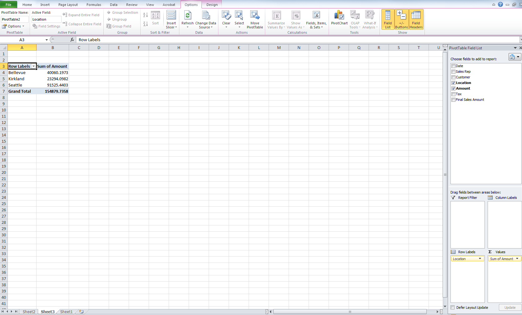
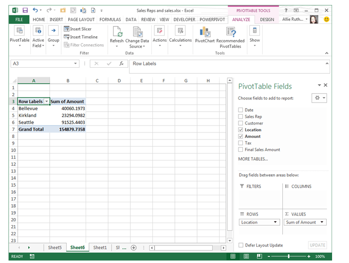
With the new Microsoft Excel-2013, you are just one click away from creating a basic pivot table. The best part is you do not have to drag and drop anything into the field list. As seen to the right, you can pull the exact information you need from a complex spreadsheet without having to go through the above mentioned steps for Excel-2010.
How do you create Pivot tables in 2013?
Instead of inserting a Pivot table from the Insert tab, just click on the “Recommended Pivot Tables” option on the Insert tab.
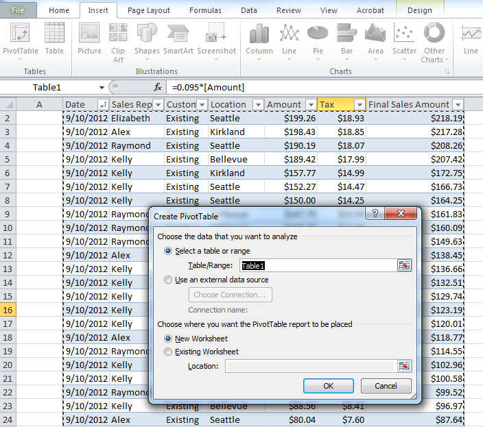
 As you can see in the above image, Excel automatically suggests three or four options for your data range. All you have to do is make sure that your cursor is in one of the data entries on the main sheet before you click on “Recommended Pivot Tables”.
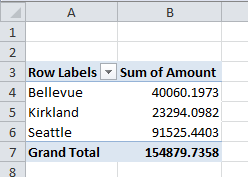
When you select one of the recommended Pivot tables, it automatically adjusts the fields without the user having to drag and drop in the Pivot table field list. Once the Pivot table is created you can customize the fields according to your requirements.
In summary, we use the following steps to create a Pivot table using Excel-2013:
1. Organize and arrange data in columns
2. Make sure each column has a heading
3. Click on Insert and select the “Recommended Pivot Charts” option
4. Choose the desired Pivot table
5. Sit back and relax
Here’s looking forward to future updates from Microsoft Office. Maybe next time Excel will be even more intuitive.

 At the end of February, we sent out a survey to all SMU staff regarding their interest in Excel training. This survey was created as all of our Spring sessions were filled to capacity the same day registration was announced! We also had a number of staff inquire about attending student-only sessions. However, those sessions were also heavily attended; therefore, we could not meet staff requests for attendance.
 Yesterday’s workshop covered the basics of Excel and an introduction to formulas. OIT will offer a