By: Rajat Shetty
Excel Pivot tables help summarize your data. They also allow you to avoid using complex formulas like Vlookup, SumIF, etc. to create a table. It can take a little while for a newbie to get the hang of Pivot tables. However, the 2013 Excel updates make creating Pivot tables even simpler.
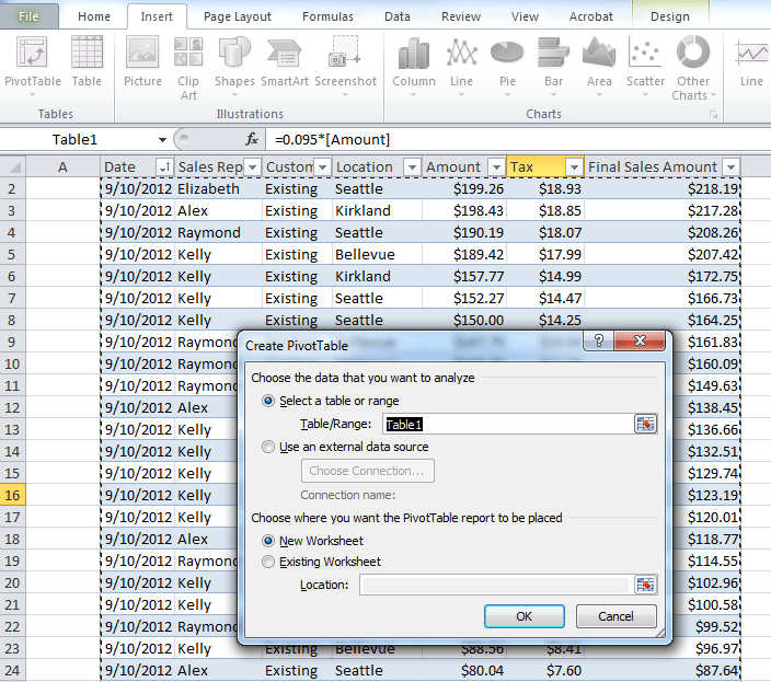
A few years back, we had to follow these steps to create a simple pivot table:
- Select the data range
- Insert pivot table from the Insert tab
- Go to the new worksheet to check if all the fields are appearing or not

4. Manually drag and drop the required fields according to our requirements to calculate-Sum, average, percentage, etc.

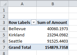
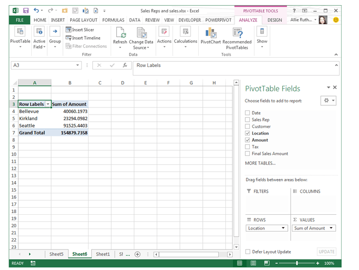
With the new Microsoft Excel-2013, you are just one click away from creating a basic pivot table. The best part is you do not have to drag and drop anything into the field list. As seen to the right, you can pull the exact information you need from a complex spreadsheet without having to go through the above mentioned steps for Excel-2010.
How do you create Pivot tables in 2013?
Instead of inserting a Pivot table from the Insert tab, just click on the “Recommended Pivot Tables” option on the Insert tab.
 As you can see in the above image, Excel automatically suggests three or four options for your data range. All you have to do is make sure that your cursor is in one of the data entries on the main sheet before you click on “Recommended Pivot Tables”.
When you select one of the recommended Pivot tables, it automatically adjusts the fields without the user having to drag and drop in the Pivot table field list. Once the Pivot table is created you can customize the fields according to your requirements.

In summary, we use the following steps to create a Pivot table using Excel-2013:
1. Organize and arrange data in columns
2. Make sure each column has a heading
3. Click on Insert and select the “Recommended Pivot Charts” option
4. Choose the desired Pivot table
5. Sit back and relax
Here’s looking forward to future updates from Microsoft Office. Maybe next time Excel will be even more intuitive.
 icon. Microsoft gives you two options you can use to insert an image. Click on the drop down arrow and either select Available Window, which gives you the option to insert another window into your document like in the example below:
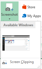 Or, you can insert a Screen Clipping, which allows you to select the specific item you want to insert. First, click on the window you want to grab the screenshot from to make the window active. Next, go back to the Office product you want to insert the screenshot into. Select the Screenshot icon and select Screen Clipping, the window that you were previously on will gray out.


 Selecting the Total Row not only adds a total line to your table, but it also has built in functions that you can toggle to further analyze specific data.

